RFDiffusion API

The RFDiffusion API runs RFDiffusion on an input template PDB file. RFDiffusion is a method for structure generation (with or without conditional information) useful for protein design challenges. RFDiffusion is capable of motif scaffolding, unconditional protein generation, symmetric motif scaffolding, binder design, and more (See References).

Examples

RFDiffusion can be run with the following command:

lev engine submit rf-diffusion input-template.pdb --n-rfdiffusion-designs 23 --n-mpnn-designs 3 --rfdiffusion-contigs A1-25/25-25 --mpnn-af2-contigs A1-25/25-25

(See Notes for more information on RFDiffusion contigs and workflow)

Inputs

• --template (str)
  • Input template PDB file
• --mpnn-af2-contigs
  • Select the contigs for the MPNN/AF2 runs
• --n-mpnn-designs
  • number of protein MPNN designs
• --n-rfdiffusion-designs
  • number of RFDiffusion designs
• --rfdiffusion-contigs
  • Contigs for RFDiffusion runs

Options

• --mpnn-model-name
  • MPNN model name to use
  • default = v_48_020
• --mpnn-model-source
  • MPNN model source [soluble, original]
  • default = soluble

Outputs

• outputs (directory)
  • Directory containing results of RFDiffusion and MPNN/AF2 runs.

Notes

Workflow

RFDiffusion contigs

The contigs flags are discussed at length in the RFdiffusion repository

README

Now, what does 'contigmap.contigs=[150-150]' mean? To those who have used RFjoint inpainting, this might look familiar, but a little bit different. Diffusion, in fact, uses the identical ‘contig mapper’ as inpainting, except that, because we’re using hydra, we have to give this to the model in a different way. The contig string has to be passed as a single-item in a list, rather than as a string, for hydra reasons and the entire argument MUST be enclosed in ‘’ so that the commandline does not attempt to parse any of the special characters.

The contig string allows you to specify a length range, but here, we just want a protein of 150aa in length, so you just specify [150-150] This will then run 10 diffusion trajectories, saving the outputs to your specified output folder.

…

In more detail, if we want to scaffold a motif, the input is just like RFjoint Inpainting, except needing to navigate the hydra config input. If we want to scaffold residues 10-25 on chain A a pdb, this would be done with 'contigmap.contigs=[5-15/A10-25/30-40]'. This asks RFdiffusion to build 5-15 residues (randomly sampled at each inference cycle) N-terminally of A10-25 from the input pdb, followed by 30-40 residues (again, randomly sampled) to its C-terminus.

References

Broadly applicable and accurate protein design by integrating prediction networks and diffusion generative models

In-depth

Introduction

RoseTTAFold Diffusion (RFDiffusion) stands out as a substantial leap forward in creating structures tailored for de novo protein design, originating from the Institute of Protein Design (IPD) at the University of Washington. They successfully used it to generate thousands of structures never before seen in nature as part of their de novo design protocol. When paired with a sequence generation tool (ProteinMPNN), they tested hundreds of structures that were shown to express well and have the desired structure and function. These innovative designs included monomers, symmetric multimers, protein binders, and enzymes.

RFDiffusion stands out for two pivotal reasons.

Firstly, it excels in producing a diverse array of protein structures with highly varied features, possessing the desired attributes. This diversity generates multiple starting hypotheses, significantly enhancing the potential for achieving the final design goal and expanding the realm of possibilities.

Secondly, RFDiffusion addresses a critical challenge in de novo design by overcoming the inherent low solubility of most novel designs. The resulting structures from RFDiffusion exhibit notable advancements in both stability and solubility, outperforming preceding methods in the field. Notably, many designs had a melting temperature above 100° C.

The groundbreaking paper introducing RFDiffusion was published on July 11, 2023, in Nature.

Since March 2023, the code has been open source, allowing our scientists at Levitate to swiftly set up, test, optimize, automate, and seamlessly integrate it for cloud computing. Drawing on our extensive experience, we not only provide implementation services but also offer valuable insights and guidance to enhance the efficiency of your protein design with RFDiffusion. Crucially, our platform equips you with essential tools to navigate efficiently through the extensive array of output models, enabling you to pinpoint optimal structures to use for the subsequent phase of de novo design (prediction of sequences for the structures generated by RFDiffusion).

Makers of RFDiffusion provide background details on github. Here, we aim to explain comprehensively for both laypeople and expert computational biologists, providing the necessary depth to empower anyone to become proficient in the subject.

Limitations

RFDiffusion will create structures for proteins with canonical amino acids. While you can use protein conformations with a desired binding mode when it is bound to small molecules or nucleotides, it does not explicitly have any way to know that the conformation should bind the small molecules or nucleotides and it will not generate these in the output models.

Note on compute costs

It’s imperative to emphasize that RFDiffusion demands significantly more computing resources compared to other AI-based protocols, exceeding the CPU time requirements of any tools in our offering. For optimal achievement of your scientific goals, we provide a dedicated document guiding the efficient utilization of this tool. After grasping the basics of RFDiffusion from this document, we strongly recommend reviewing the RFDiffusion Costs document before proceeding.

Simple example

The minimal input needs only to define how large your output protein should be. For example, you can tell it to make a protein 50 to 100 residues long. It will randomly select a number from 50 to 100 and create a protein that size. It could be mostly-helix, beta-sheet, or a combination of both, just like native proteins. It is normal to have it generate hundreds to thousands of repeats of the protocol to have a diverse output to choose from. However, this simple example has very limited applicability.

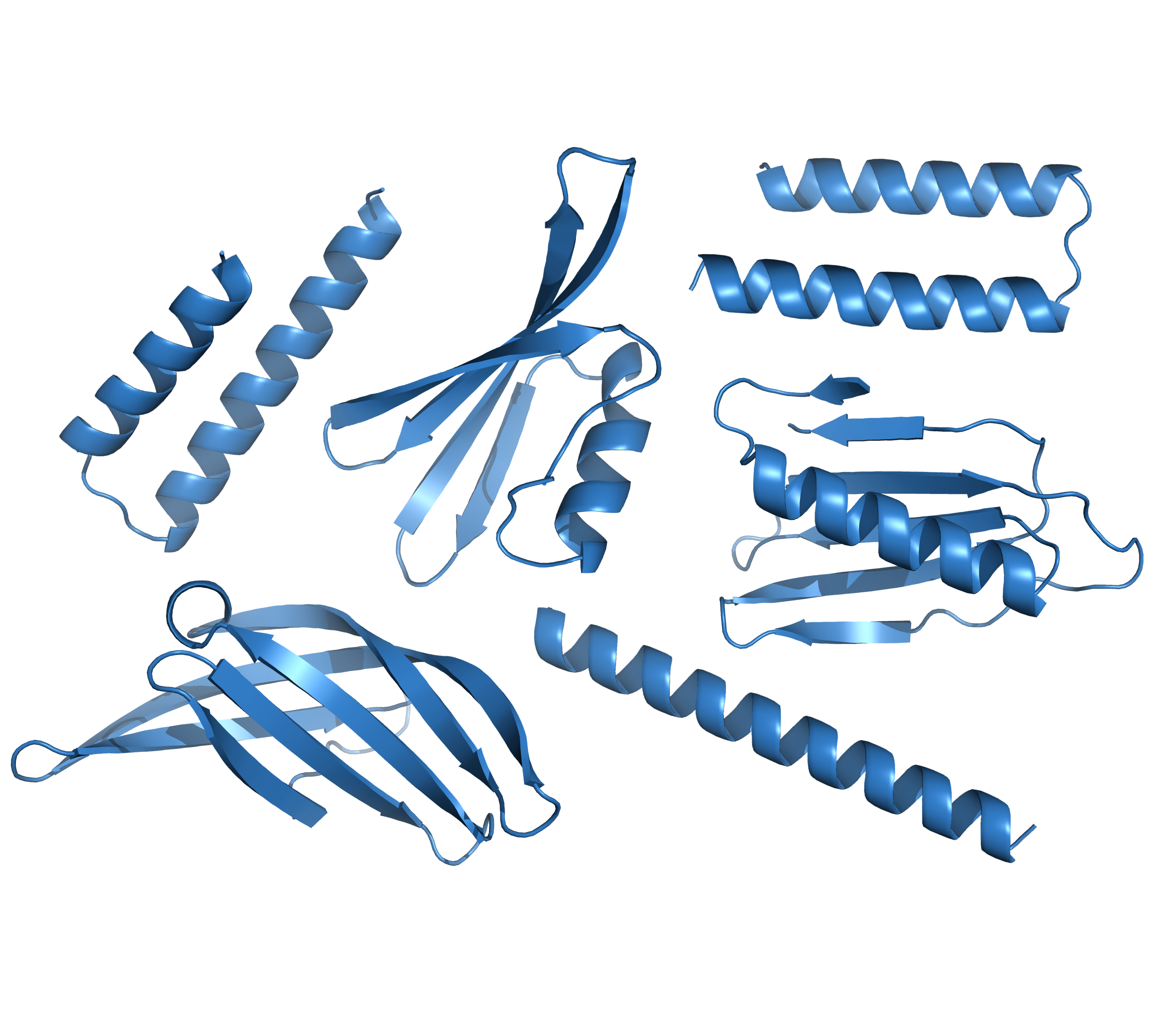
Below are random examples of RFDiffusion models. While some appear reasonable, others may not exhibit entirely native-like characteristics. For instance, the generation of a single long helix is a common occurrence with RFDiffusion which is unlikely to work for most design goals. It’s advisable to anticipate that most structures won’t align with your desired features. Planning to create numerous structures and investing time in filtering the output to select the best hits for the next step is recommended. Further guidance on filtering will be elaborated in the filtering section below.

Simple binder example

A more common example is if you have a target protein and wish to create a new protein that binds it at a specific site. For this example, your inputs could be:

• The target protein structure in a PDB
• The residues in the PDB that will be retained for the modeling process and will be in the output models
• The positions on the structure where you want the new protein to bind
• A range of sizes that you want the new protein to have
  • Providing a range of sizes allows for more diversity of hallucinated new proteins
• The number of repeats you want to be created
  • Run a single RFDiffusion if you want to get an idea of how your variables run.
  • Run a small set with 100 repeats to have a reasonable range of options for a very simple design if you don’t expect it to be challenging.
  • Run 1k to 5k repeats to better explore the search space. You may need to run 10 RFDiffusions with 5k repeats each for very challenging goals.

That example will output a set of PDBs that have the hallucinated proteins bound to your original protein and the binding site should be in the region that you indicated. The novel protein will only have glycine residues, so you must run MPNN to generate sequences that will fold into the desired conformation.

The new protein is predicted to be stable and soluble on its own but binds to the target protein when present. However, it’s essential to acknowledge that, in practice, not every protein generated by RFDiffusion possesses the potential to become a stable, expressed protein. The details of this aspect are elaborated upon in the subsequent filtering section.

Adding residues to increase or create binding to a target protein

Many design challenges involve a protein-protein interaction that is not strong enough even though interface mutations have been extensively explored. Another way to increase binding and specificity is to add on to a protein interaction. In this example, you are starting with a PDB that has a protein-protein interaction present and you want to extend one of the proteins to have a larger interaction. Or, you could even have two proteins in a PDB that are over 15 angstroms away from each other in the PDB and let RFDiffusion create the binding site.

In this example, you have a “design” protein that you want to add onto which will be structurally compatible with the design protein and create interactions with a “target” protein. So you will hallucinate an additional section of the design protein. Your inputs would be:

• The PDB with both proteins present in the conformation you want them to end up in - Meaning, RFDiffusion is not expected to shift the two proteins to help make them bind as it runs RFDiffusion. It will fill in a hallucinated section that creates a new section of the design protein to create the interaction.
• Indicate which parts of both proteins in the file are expected to stay in the model.
• Indicate where you want the hallucination to occur in the design protein.
  • Meaning, you will be adding residues to the design protein and you need to define exactly where in the sequence it will be inserted.
  • Easy locations: N or C ends, or in the middle of a loop.
  • Not recommended in the middle of a helix of beta-sheet because it will be more challenging to generate a compatible structure.
  • You can insert hallucinated residues in multiple places.
• The positions on the structure where you want the hallucinated protein to bind to the target protein
• A range of sizes that you want the new protein to have
• The number of repeats you want to be created

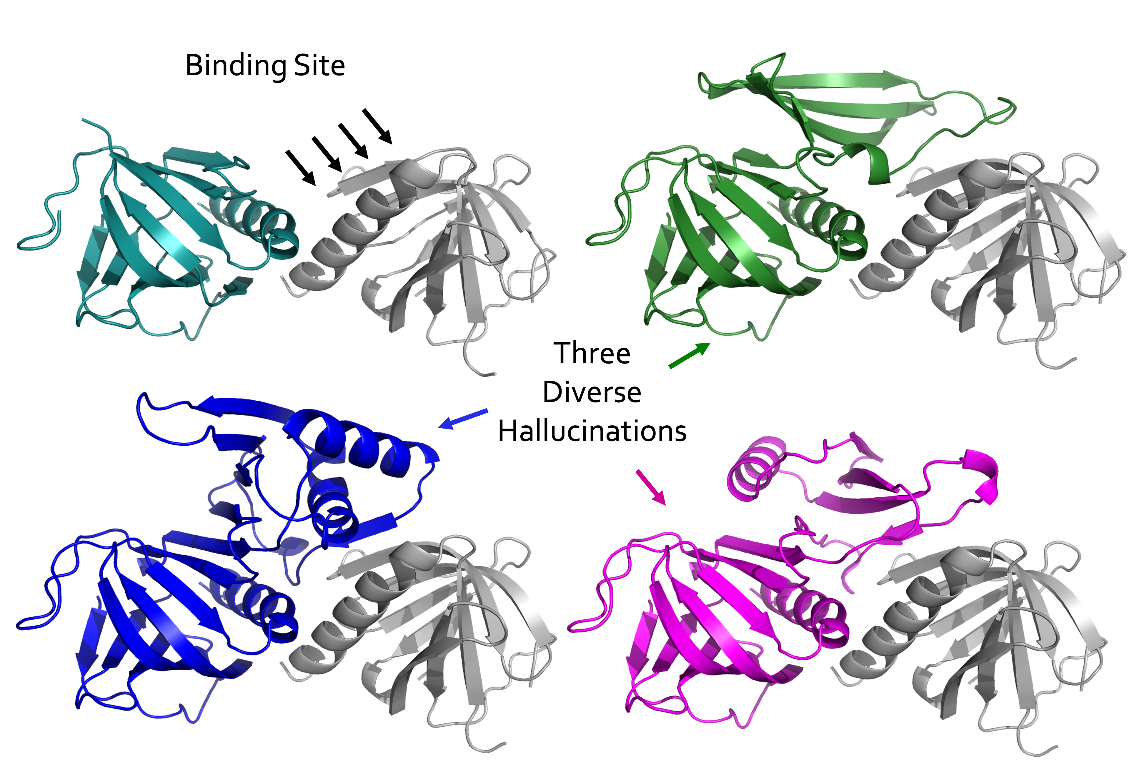
Below is an example where residues are hallucinated to expand the binding of one protein to another. In the top left corner, the design protein is in teal and the target protein is grey. We ran RFDiffusion and told it to insert 50 to 100 residue section in the middle of a loop of the design protein that will create binding at the indicated site. The structures in green, purple, and blue are 3 diverse designs created by RFDiffusion.

Creating a binder using a binding motif

Like the last example, this involves having a protein and wishing to create a new protein that binds it at a specific site. However, in this scenario, you already possess information about a protein or peptide that binds to the desired site.

You should have a PDB file containing the target protein bound to a protein with the desired binding motif. The motif can be an entire secondary structure involved in binding or specific segments of the protein that may not necessarily be contiguous. For instance, if two loops contribute to the binding process, both can be included in the motif. Alternatively, you have the flexibility to choose individual non-contiguous residues that maintain a conformation deemed crucial for binding.

When the motif is not continuous, the challenge is to decide how the hallucinated regions should be inserted. It is straightforward to allow hallucinations on the N and/or C ends of a motif.

However, if you have a binding motif like the following example, there are many solutions. Below is a target protein bound to a protein with a desired binding motif in A. You can select one entire section like in B. In which case your can add hallucinated protein residues on one or both ends to generate a protein with that motif. In C, we have selected individual residues in that binding site to retain in the motif. For B, we have selected two continuous motifs that have a significant distance from each other.

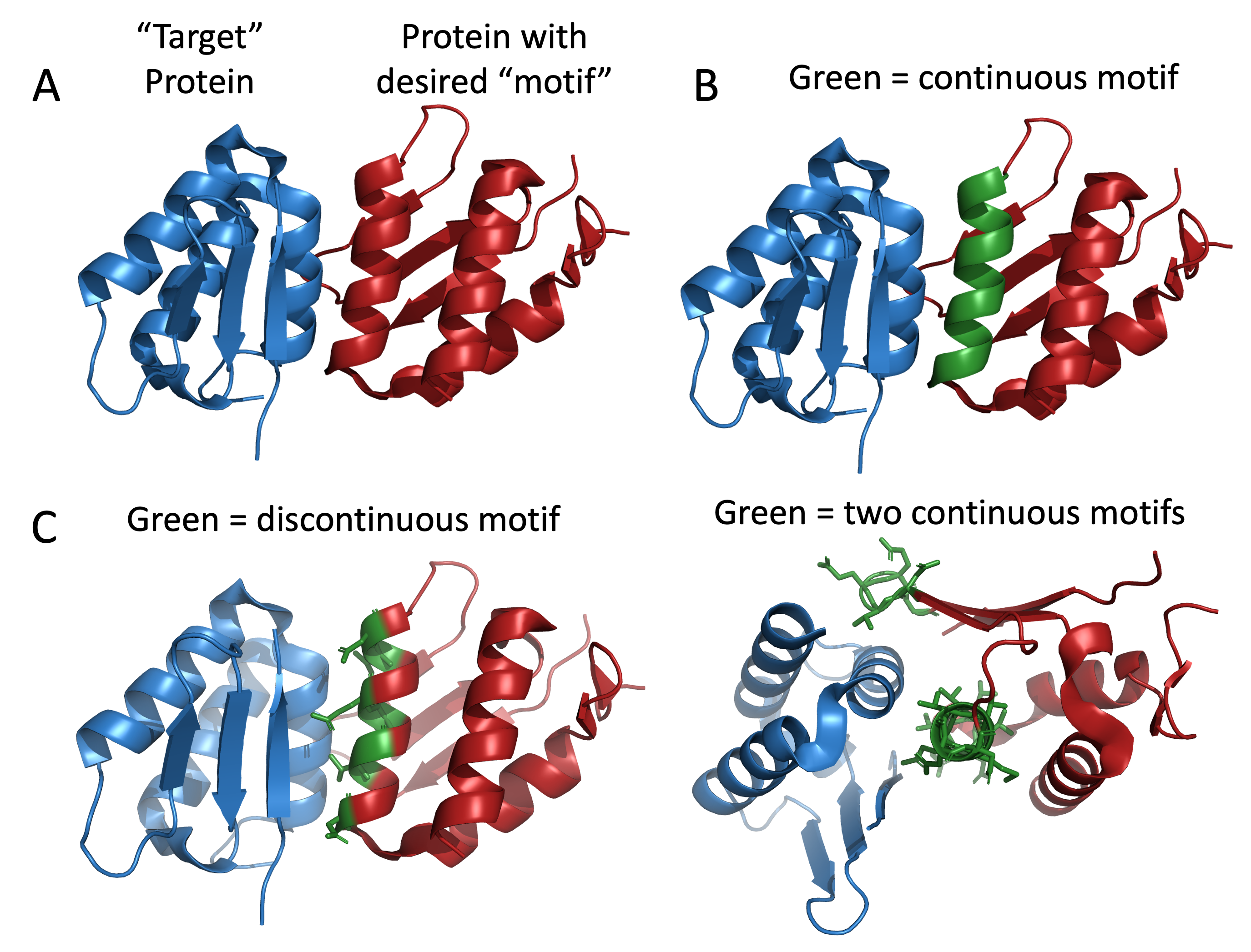
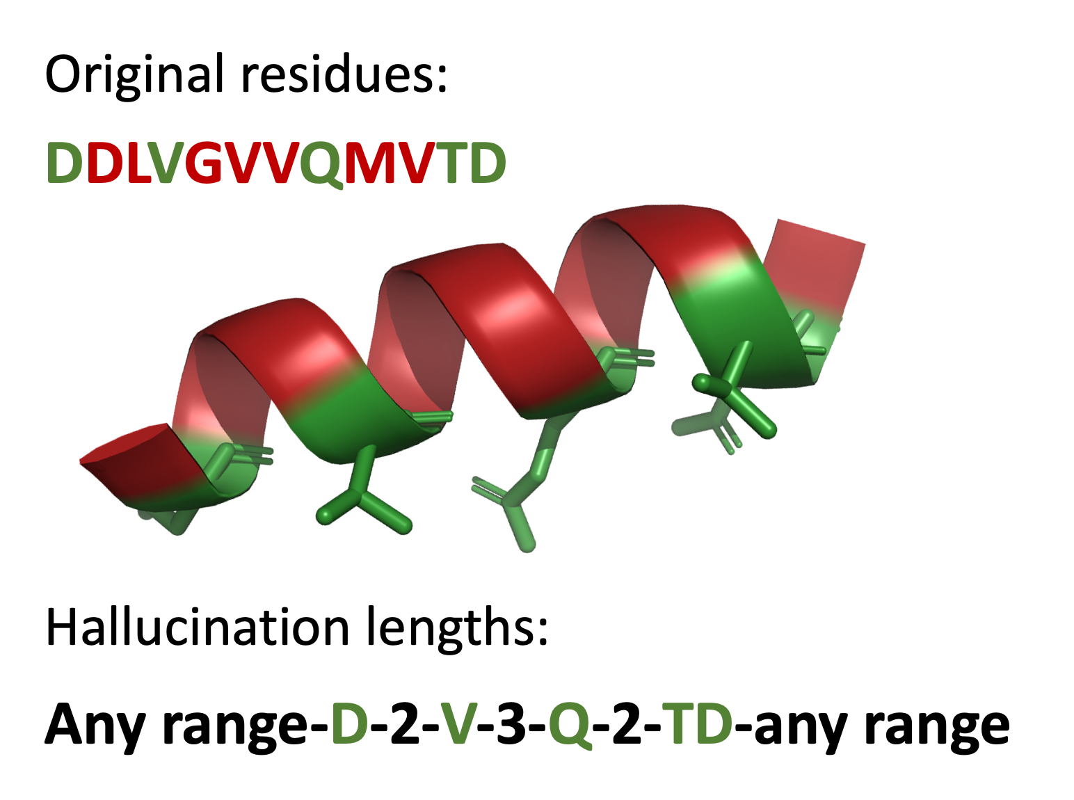
Why opt for the example in C instead of B? In C, these residues can only maintain this conformation if they are part of a helix identical or very similar to B. The question arises: why bother? Consider the helix having two sides – a binding side and a side involved in packing into the protein core. While the core side evolved for optimal packing in this protein, our goal is to alter the core. Allowing RFDiffusion to hallucinate the backbone for the core side of the helix broadens the range of cores it can imagine. However, it’s essential to inform RFDiffusion of the correct number of residues between those in C to ensure accurate helix construction, as illustrated below.

Your inputs:

• The PDB with the target protein bound to the protein with the binding motif
• Indicate which parts of both proteins in the file are expected to stay in the model.
  • The “motif” section in the design protein is all that needs to be retained for this example
  • The domain of the target protein involved in binding should be retained
• Indicate where you want the hallucination to occur in relation to the motif.
  • Meaning, you need to define where in the hallucinated protein the motif can occur.
  • For a single continuous motif, you can have protein before and/or after the motif.
  • For discontinuous motifs, you also need to define the positions between the residues.
• A range of sizes that you want the new protein to have
• The number of repeats you want created

Creating a simple monomer

Vanilla RFDiffusion is the default version that generates monomeric proteins without specifying conditions other than their size and the number of output models that you want.

For example, the command might look like this:

lev engine submit rf-diffusion --n-rfdiffusion-designs 50 --rfdiffusion-contigs='[50-100]'

• --n-rfdiffusion-designs 50
  • Flag needed to define # of output models as 50
• --rfdiffusion-contigs='[50-100]'
  • Flag needed to define the range of protein lengths that it will create as 50 to 100 residues long
  • If you want a single length: '[50-50]'

Creating a simple binder

If you have a target protein and wish to create a new protein that binds it at a specific site. The command might look like this:

lev engine submit rf-diffusion input.pdb --n-rfdiffusion-designs 50 --rfdiffusion-contigs='[50-100\0 B1-50]' --custom-arguments='ppi.hotspot_res=[B26,B28,B30]'

• --n-rfdiffusion-designs 50
  • Flag needed to define # of output models as 50
• --rfdiffusion-contigs='[50-100\0 B1-50]'
  • Flag needed to define the expected linear features for the output models.
• The first part of the output models will contain hallucinated protein and will have 50 to 100 hallucinated residues (since a chain letter is not present).
• \0 indicates that the next section is the end of the first protein that will be in the output models, but not necessarily the end of the proteins that will be in the output.

• B1-50 indicates that the next part of the output will be residues 1 to 50 of chain B from input.pdb.

• --custom-arguments='ppi.hotspot_res=[B26,B28,B30]'
  • Flag needed to define the binding site that the new residues should interact with.
  • --custom-arguments= is a general flag indicating a variable will be added
  • ppi.hotspot_res is the argument for the flag indicating that the hallucinated residues should have some interactions generated.
  • [B26,B28,B30] indicates the positions from input.pdb protein/proteins where it should create interactions.

Extending a protein to improve or create binding

If you have two proteins that you want to bind or to bind better by extending to total length of the first protein, the command might look like this:

lev engine submit rf-diffusion input.pdb --n-rfdiffusion-designs 50
--rfdiffusion-contigs='[A1-25/50-100/A26-100\0 B1-50]'
--custom-arguments='ppi.hotspot_res=[B26,B28,B30]'

• --n-rfdiffusion-designs 50
  • Flag needed to define # of output models as 50
• --rfdiffusion-contigs='[A1-25/50-100/A26-100\0 B1-50]'
  • Flag needed to define the expected linear features for the output models.
  • The first part of the output models will contain the residues 1 to 25 of chain A from input.pdb as indicated by A1-25
  • / indicates the next section is inserted in the output models.
  • 50-100 indicates that the next part of the output models will have 50 to 100 hallucinated residues (since a chain letter is not present).
  • /A26-100 indicates that the next section will be chain A residues 26 to 100.
  • 0 indicates that the next section is the end of the first protein that will be in the output models, but not necessarily the end of the proteins that will be in the output.
  • B1-50 indicates that the next part of the output will be residues 1 to 50 of chain B from input.pdb.
• --custom-arguments='ppi.hotspot_res=[B26,B28,B30]
  • Flag needed to define the binding site that the new residues should interact with.
• --custom-arguments=
  • Flag indicating a variable will be added
• ppi.hotspot_res
  • The argument for the flag indicating that the hallucinated residues should have some interactions generated.
• [B26,B28,B30]
  • Indicates the positions from input.pdb protein/proteins where it should create interactions.

Creating a binder using a motif

If you have a region of a protein (contiguous or noncontiguous) that you want to keep in the output models, it just needs to be included in the contigs list. For example, you can have a PDB with 2 bound proteins. The first protein has a single helix (chain A residues 22-31) involved in binding that you want to keep. And you want it to be extended on both ends to form a new protein. And you want additional binding to protein B. The command might look like this:

lev engine submit rf-diffusion input.pdb --n-rfdiffusion-designs 50
--rfdiffusion-contigs='[10-50/A22-31/10-500 B1-50]' --custom-arguments='ppi.hotspot_res=[B26,B28,B30]'

• --n-rfdiffusion-designs 50
  • Flag needed to define # of output models as 50
• --rfdiffusion-contigs='[10-50/A22-31/10-500 B1-50]'
  • Flag needed to define the expected linear features for the output models.
• 10-50 indicates that the first part of the output models will contain 10 to 50 hallucinated residues
• /A22-31 indicates that the next part of the protein will be the helix from chain A from input.pdb.
• 10-500 indicates that the last section of the protein will contain 10 to 500 hallucinated residues
• B1-50 indicates that the next part of the output will be residues 1 to 50 of chain B from input.pdb.
• --custom-arguments='ppi.hotspot_res=[B26,B28,B30]'
  • Flag needed to define the binding site that the new residues should interact with.
• --custom-arguments='' is a general flag indicating a variable will be added
• ppi.hotspot_res is the argument for the flag indicating that the hallucinated residues should have some interactions generated.
• [B26,B28,B30] indicates the positions from input.pdb protein/proteins where it should create interactions.

Filtering output models

While RFDiffusion produces diverse models, not all may align with your goals, prompting the need for a filtering process.

Using Radius of Gyration for Compactness:

• The Radius of Gyration tool assess how tightly packed the protein structures are.
• Stable, soluble protein typically has tighter packing and has a lower Radius of Gyration.
• Visually inspect the output models to establish favorable Radius of Gyration scores and filter out those with less favorable scores.

Filtering Models with Ratio of Loops-Helices-Sheets:

• Rosetta can measure the ratio of loops, helices, and beta sheets in models.
• Excessive amount of loops can lead to instability.
• Visually inspect the output models to establish favorable ratio of loops and filtering out those with less favorable ratios.
• Ratio data can also help select diverse structures to use for subsequent steps.

Selection Based on Binding Site:

• Rosetta’s Interface Analyzer can pull relevant data on binding interfaces.
• If designing a binding protein, focus on models with optimal interface packing and interface surface area.
• Some of its output will not be relevant for polyglicines that will later be mutated, such as # of hydrogen bonds and # of unpaired polar atoms.

Clustering for Structural Similarity:

• Calculate Root Mean Square Deviation (RMSD) between all output models to create a distance matrix.
• Cluster models based on structural similarity.
• Visually inspect each cluster’s representative models and select those that appear reasonable for the next design phase, ProteinMPNN.

You can use one or several of the models from an RFDiffusion run as input for ProteinMPNN. It is often advisable to use a diverse range of models to see which appears to be generating good results. The hallucinated portion of RFDiffusion’s output models will be polyglycine and ProteinMPNN will hallucinate sequence that it predicts will fold into the input structure.

See our ProteinMPNN documentation for more details.